CCA Tutorial

This tutorial demonstrates the use of CCA for 2 views and multiview CCA (MCCA) for more than 2 views. As is demonstrated, they allow for both the addition of regularization as well as the use of a kernel to compute the distance (Gram) matrices (KMCCA).

# Authors: Iain Carmichael, Ronan Perry
# License: MIT

from mvlearn.datasets import sample_joint_factor_model
from mvlearn.embed import CCA, MCCA, KMCCA
from mvlearn.plotting import crossviews_plot


n_views = 3
n_samples = 1000
n_features = [10, 20, 30]
joint_rank = 3

# sample 3 views of data from a joint factor model
# m, noise_std control the difficulty of the problem
Xs, U_true, Ws_true = sample_joint_factor_model(
    n_views=n_views, n_samples=n_samples, n_features=n_features,
    joint_rank=joint_rank, m=5, noise_std=1, random_state=23,
    return_decomp=True)

CCA

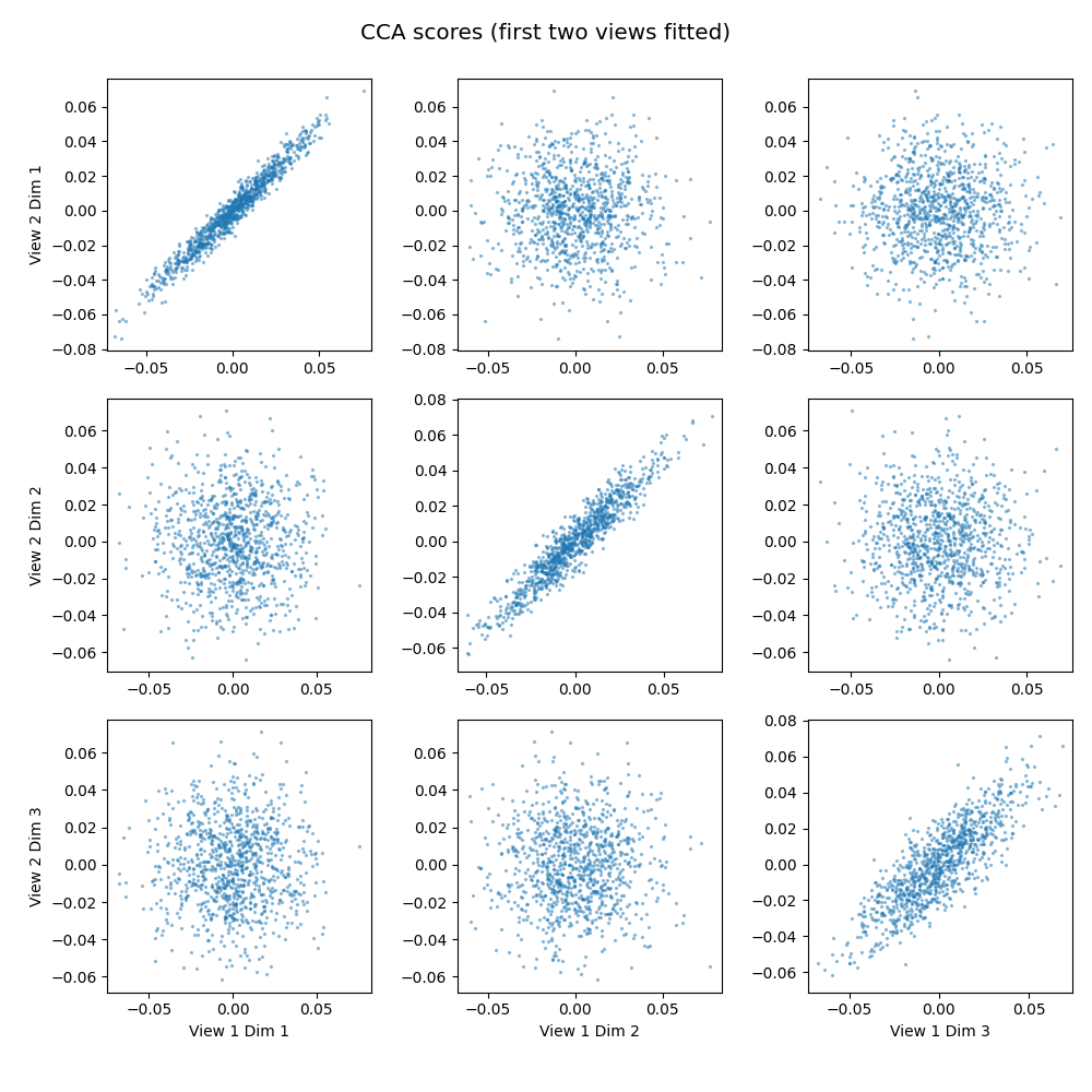
CCA, equivalent to 2 view MCCA, learns transformations of the views, projecting a linear combination of the features to a component such that the sum of correlations between the ith components of each view is maximized. We see the top three components of the first two views plotted against each other, pairwise. The strong linear shape on the diagonals shows that the found components correlate well.

# the default is no regularization meaning this is SUMCORR-AVGVAR MCCA
cca = CCA(n_components=joint_rank)

# the fit-transform method outputs the scores for each view
cca_scores = cca.fit_transform(Xs[:2])
crossviews_plot(cca_scores,
                title='CCA scores (first two views fitted)',
                equal_axes=True,
                scatter_kwargs={'alpha': 0.4, 's': 2.0})

# In the 2 view setting, a variety of interpretable statistics can be
# calculated. We assess the canonical correlations achieved and
# their significance using the p-values from a Wilk's Lambda test

stats = cca.stats(cca_scores)
print(f'Canonical Correlations: {stats["r"]}')
print(f'Wilk\'s Lambda Test pvalues: {stats["pF"]}')

Out:

Canonical Correlations: [0.97683992 0.94623958 0.83236882]
Wilk's Lambda Test pvalues: [1.11022302e-16 1.11022302e-16 1.11022302e-16]

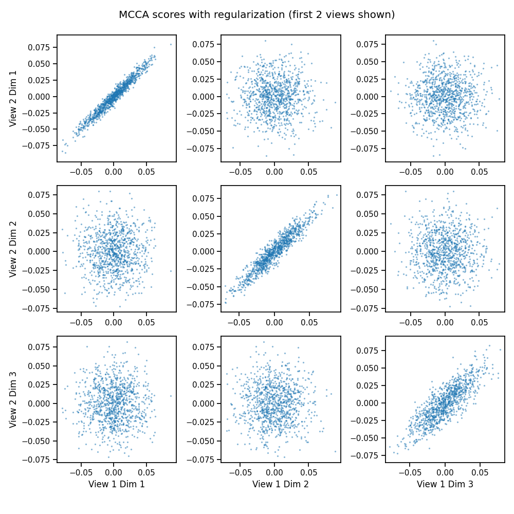
Regularized CCA

We can add regularization with the regs argument to handle high-dimensional data. This data is simple, and so it makes little difference. Here, we use MCCA for all 3 views.

# regularization value of .5 for each view
mcca = MCCA(n_components=joint_rank, regs=0.5)

# the fit-transform method outputs the scores for each view
mcca_scores = mcca.fit_transform(Xs)
crossviews_plot(mcca_scores[[0, 1]],
                title='MCCA scores with regularization (first 2 views shown)',
                equal_axes=True,
                scatter_kwargs={'alpha': 0.4, 's': 2.0})

print('Canonical Correlations:')
print(mcca.canon_corrs(mcca_scores))

Out:

Canonical Correlations:
[[[1.         0.97667891 0.97566468]
  [0.97667891 1.         0.97828026]
  [0.97566468 0.97828026 1.        ]]

 [[1.         0.94580941 0.94498116]
  [0.94580941 1.         0.94657566]
  [0.94498116 0.94657566 1.        ]]

 [[1.         0.83109131 0.82482284]
  [0.83109131 1.         0.82443132]
  [0.82482284 0.82443132 1.        ]]]

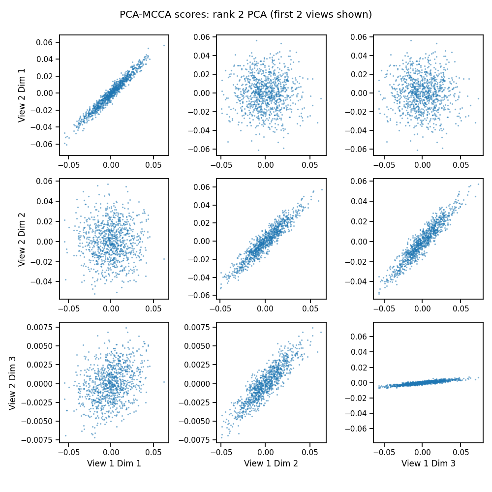
Informative MCCA: PCA then MCCA

We can also handle high-dimensional data with i-MCCA. We first compute a low rank PCA for each view, then run MCCA on the reduced data. With rank 2 PCA, only the first two CCA components are informative, as we can see in the plot.

# i-MCCA where we first extract the first 2 PCs from each data view
mcca = MCCA(n_components=joint_rank, signal_ranks=[2, 2, 2])

mcca_scores = mcca.fit_transform(Xs)
crossviews_plot(mcca_scores[[0, 1]],
                title='PCA-MCCA scores: rank 2 PCA (first 2 views shown)',
                equal_axes=True,
                scatter_kwargs={'alpha': 0.4, 's': 2.0})

print('Canonical Correlations:')
print(mcca.canon_corrs(mcca_scores))

Out:

Canonical Correlations:
[[[ 1.          0.97612813  0.97510341]
  [ 0.97612813  1.          0.97754325]
  [ 0.97510341  0.97754325  1.        ]]

 [[ 1.          0.94495697  0.94345871]
  [ 0.94495697  1.          0.94470975]
  [ 0.94345871  0.94470975  1.        ]]

 [[ 1.          0.88039793 -0.94276507]
  [ 0.88039793  1.         -0.89227834]
  [-0.94276507 -0.89227834  1.        ]]]

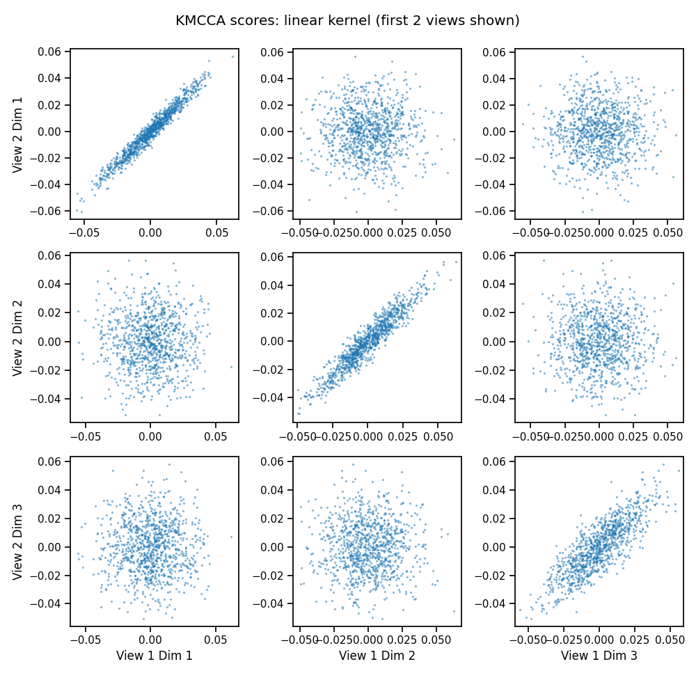
Kernel MCCA

We can compute kernel MCCA with the KMCCA() object. With the linear kernel, this behaves just like MCCA.

# fit kernel MCCA with a linear kernel
kmcca = KMCCA(n_components=joint_rank, kernel='linear')

kmcca_scores = kmcca.fit_transform(Xs)
crossviews_plot(kmcca_scores[[0, 1]],
                title='KMCCA scores: linear kernel (first 2 views shown)',
                equal_axes=True,
                scatter_kwargs={'alpha': 0.4, 's': 2.0})

print('Canonical Correlations:')
print(mcca.canon_corrs(mcca_scores))

Out:

Canonical Correlations:
[[[ 1.          0.97612813  0.97510341]
  [ 0.97612813  1.          0.97754325]
  [ 0.97510341  0.97754325  1.        ]]

 [[ 1.          0.94495697  0.94345871]
  [ 0.94495697  1.          0.94470975]
  [ 0.94345871  0.94470975  1.        ]]

 [[ 1.          0.88039793 -0.94276507]
  [ 0.88039793  1.         -0.89227834]
  [-0.94276507 -0.89227834  1.        ]]]