Partial Gram-Schmidt Orthogonalization (PGSO) for KMCCA

Kernel matrices grow exponentially with the size of the data. There are immense storage and run-time constraints that arise when working with large datasets. The partial Gram-Schmidt orthogonalization (PGSO) finds a low-rank approximation of the Cholesky decomposition of the kernel matrix. This reduces storage requirements from O(n^2) to O(nm), where n is the number of subjects (rows) and m is the rank of the kernel matrix. This also reduces the run-time from O(n^3) to O(nm^2).

# Authors: Ronan Perry, Theodore Lee
# License: MIT

import timeit
import numpy as np
import matplotlib.pyplot as plt
from mvlearn.plotting.plot import crossviews_plot
from mvlearn.embed import KMCCA
import warnings
warnings.filterwarnings("ignore")


def make_data(N, seed=None):
    np.random.seed(seed)
    t = np.random.uniform(-np.pi, np.pi, N)
    e1 = np.random.normal(0, 0.1, (N, 2))
    e2 = np.random.normal(0, 0.1, (N, 2))

    X1 = np.zeros((N, 2))
    X1[:, 0] = t
    X1[:, 1] = np.sin(3*t)
    X1 += e1

    X2 = np.zeros((N, 2))
    X2[:, 0] = np.exp(t/4)*np.cos(2*t)
    X2[:, 1] = np.exp(t/4)*np.sin(2*t)
    X2 += e2

    return [X1, X2]

Full Decomposition vs PGSO on Sample Data

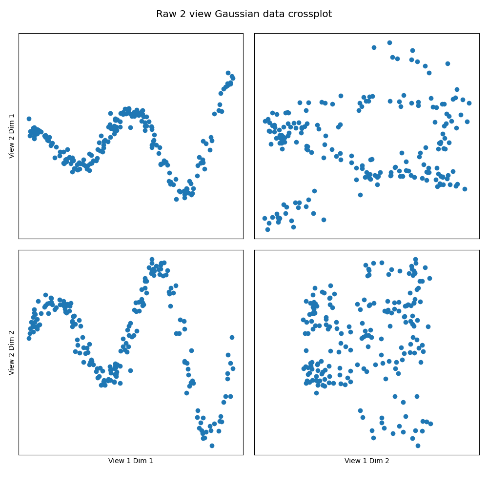
PGSO is run on two views of data that each have two dimensions that are sinuisoidally related. The data has 100 samples and thus the fully decomposed kernel matrix would have dimensions (100, 100). PSGO finds an approximation with lower rank at the given tolerance of 0.5 to the full kernel matrix.

Xs_train = make_data(100, seed=1)
Xs_test = make_data(200, seed=2)


crossviews_plot(Xs_test, ax_ticks=False, ax_labels=True, equal_axes=True,
                title='Raw 2 view Gaussian data crossplot')

Full Decomposition

kmcca = KMCCA(kernel="rbf", n_components=2, regs=0.01)
scores = kmcca.fit(Xs_train).transform(Xs_test)

crossviews_plot(scores, ax_ticks=False, ax_labels=True, equal_axes=True,
                title='KMCCA scores (full decomposition)')

corrs = kmcca.canon_corrs(scores)

print("The first two canonical correlations are "
      f"[{corrs[0]:.3f}, {corrs[1]:.3f}]")

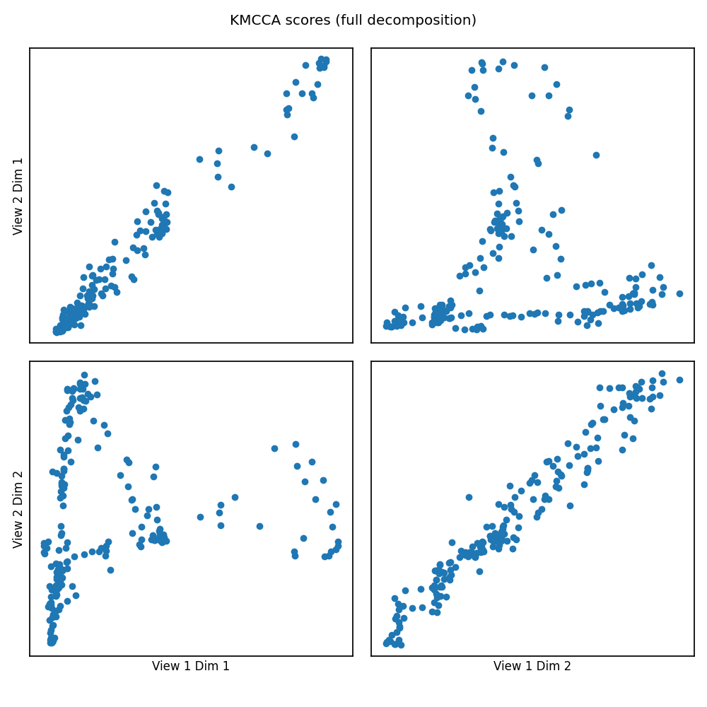
Out:

The first two canonical correlations are [0.987, 0.977]

PGSO Decomposition

kmcca = KMCCA(kernel="rbf", n_components=2, regs=0.01, pgso=True)
scores = kmcca.fit(Xs_train).transform(Xs_test)

crossviews_plot(scores, ax_ticks=False, ax_labels=True, equal_axes=True,
                title='KMCCA scores (PGSO decomposition)')

corrs = kmcca.canon_corrs(scores)

print("The first two canonical correlations are "
      f"[{corrs[0]:.3f}, {corrs[1]:.3f}], at ranks "
      f"{kmcca.pgso_ranks_}")

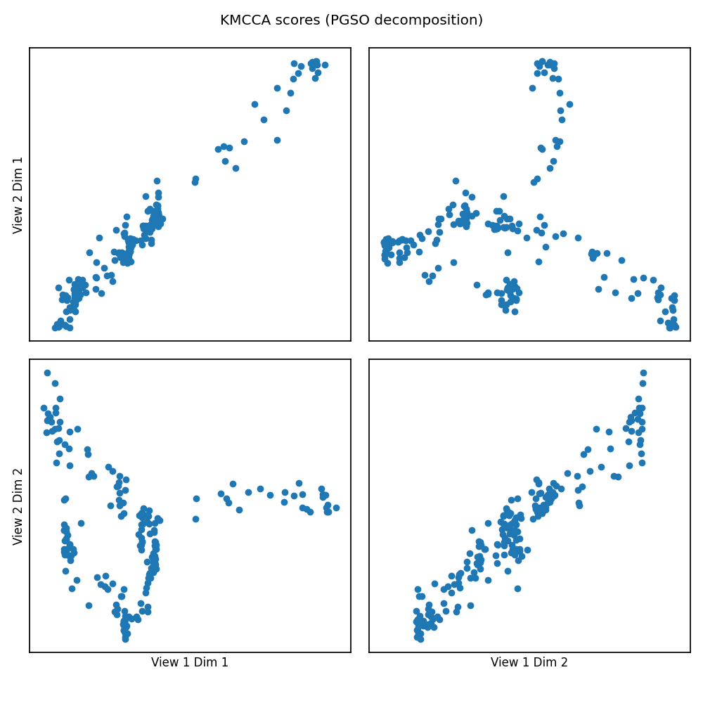
Out:

The first two canonical correlations are [0.984, 0.958], at ranks [10, 8]

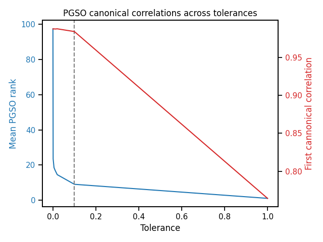
PGSO Tolerance vs. Canonical Correlation and Rank

We can observe the relationship between the PGSO tolerance and canonical correlation of the first canonical component as well as the approximation rank.

We observe that at tol=0.1, the mean rank is approximately 15 and yet we achieve similarly high canonical correlation as with the full kernel matrix.

canon_corrs = []
ranks = []
tols = [0, 0.001, 0.005, 0.01, 0.02, 0.1, 1]
for p in tols:
    kmcca = KMCCA(kernel="rbf", n_components=2, regs=0.01, pgso=True,
                  tol=p)
    scores = kmcca.fit(Xs_train).transform(Xs_test)
    corrs = kmcca.canon_corrs(scores)
    canon_corrs.append(corrs[0])
    ranks.append(np.mean(kmcca.pgso_ranks_))

fig, ax1 = plt.subplots()

color = 'tab:blue'
ax1.set_ylabel('Mean PGSO rank', color=color)
ax1.set_xlabel('Tolerance')
ax1.plot(tols, ranks, color=color)
ax1.tick_params(axis='y', labelcolor=color)
ax1.axvline(0.1, ls='--', c='grey')

color = 'tab:red'
ax2 = ax1.twinx()
ax2.set_ylabel('First cannonical correlation', color=color)
ax2.plot(tols, canon_corrs, color=color)
ax2.tick_params(axis='y', labelcolor=color)

plt.title('PGSO canonical correlations across tolerances')
plt.tight_layout()
plt.show()

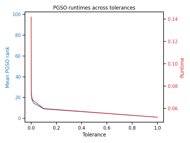
PGSO Tolerance vs. Runtime and Rank

We can observe the relationship between the PGSO tolerance and the run-time fit and transform the two views (separately). We average the run-time of each rank over multiple trials.

From the rank vs canonical correlation analysis in the previous section, we discovered that a tolerance of 0.1 will preserve the canonical correlation (accuracy). We also see here that we can get an order of magnitude decrease in run-time compared to the full decomposition (tolerance 0).

runtimes = []
ranks = []
for p in tols:
    kmcca = KMCCA(kernel="rbf", n_components=2, regs=0.01, pgso=True,
                  tol=p)
    runtime = timeit.timeit(
        lambda: kmcca.fit(Xs_train).transform(Xs_test), number=10)
    runtimes.append(runtime)
    ranks.append(np.mean(kmcca.pgso_ranks_))

fig, ax1 = plt.subplots()

color = 'tab:blue'
ax1.set_ylabel('Mean PGSO rank', color=color)
ax1.set_xlabel('Tolerance')
ax1.plot(tols, ranks, color=color)
ax1.tick_params(axis='y', labelcolor=color)

color = 'tab:red'
ax2 = ax1.twinx()
ax2.set_ylabel('Runtime', color=color)
ax2.plot(tols, runtimes, color=color)
ax2.tick_params(axis='y', labelcolor=color)

plt.title('PGSO runtimes across tolerances')
plt.tight_layout()
plt.show()