Multiview vs. Singleview Spectral Clustering of UCI Multiview Digits

Here, we directly compare multiview methods available within mvlearn to analagous singleview methods. Using the UCI Multiple Features Dataset, we first examine the dataset by viewing it after using dimensionality reduction techniques, then we perform unsupervised clustering and compare the results to the analagous singleview methods.

# Authors: Gavin Mischler, Ronan Perry
#
# License: MIT

from sklearn.cluster import SpectralClustering
from sklearn.metrics import homogeneity_score
from mvlearn.cluster import MultiviewSpectralClustering
from mvlearn.embed import MVMDS
from sklearn.decomposition import PCA
from sklearn.metrics import confusion_matrix
from mvlearn.datasets import load_UCImultifeature
import numpy as np
import matplotlib.pyplot as plt
from mpl_toolkits.axes_grid1 import make_axes_locatable

Load and visualize the multiple handwritten digit views

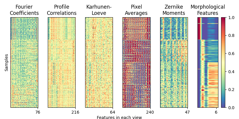
We load a 6-view, 4-class dataset from the Multiple Features Dataset. Each of the six views are as follows:

1. 76 Fourier coefficients of the character shapes

2. 216 profile correlations

3. 64 Karhunen-Love coefficients

4. 240 pixel averages of the images from 2x3 windows

5. 47 Zernike moments

6. 6 morphological features

Xs, y = load_UCImultifeature(select_labeled=[0, 1, 2, 3])
view_names = ['Fourier\nCoefficients', 'Profile\nCorrelations',
              'Karhunen-\nLoeve', 'Pixel\nAverages',
              'Zernike\nMoments', 'Morphological\nFeatures']

order = np.argsort(y)
sub_samp = np.arange(0, Xs[0].shape[0], step=3)

fig, axes = plt.subplots(1, 6, figsize=(8, 4))
for i, view in enumerate(Xs):
    sorted_view = view[order, :].copy()
    sorted_view = sorted_view[sub_samp, :]

    # Scale features in each view to [0, 1]
    minim = np.min(sorted_view, axis=0)
    maxim = np.max(sorted_view, axis=0)
    sorted_view = (sorted_view - minim) / (maxim - minim)

    pts = axes[i].imshow(
        sorted_view, cmap='Spectral_r', aspect='auto', vmin=0, vmax=1)

    axes[i].set_title(view_names[i], fontsize=12)
    axes[i].set_yticks([])
    max_dim = view.shape[1]
    axes[i].set_xticks([max_dim-1])
    axes[i].set_xticklabels([str(max_dim)])

divider = make_axes_locatable(axes[-1])
cax = divider.append_axes("right", size="20%", pad=0.1)
plt.colorbar(pts, cax=cax)
fig.text(0.5, 0, 'Features in each view', ha='center')
axes[0].set_ylabel('Samples')
plt.tight_layout()
plt.show()

Comparing dimensionality reduction techniques

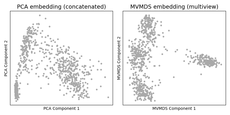
As one might do with a new dataset, we first visualize the data in 2 dimensions. The naive approach using singleview method would be to concatenate the views and apply PCA. Ung the multiview Multi-dimensional Scaling (mvlearn.embed.MVMDS) available in the package we can jointly embed the views to find their common principal components across views.

A visual inspection of the resulting embeddings see that MVMDS better finds four separate groups. With PCA, it is less clear how many clusters there are in the data.

Xs_mvmds = MVMDS(n_components=2).fit_transform(Xs)
Xs_pca = PCA(n_components=2).fit_transform(np.hstack(Xs))

sca_kwargs = {'s': 10, 'color': 'darkgray'}
f, axes = plt.subplots(1, 2, figsize=(8, 4))
axes[0].scatter(Xs_pca[:, 0], Xs_pca[:, 1], **sca_kwargs)
axes[0].set_title('PCA embedding (concatenated)', fontsize=14)
axes[0].set_xlabel('PCA Component 1')
axes[0].set_ylabel('PCA Component 2')
axes[1].scatter(Xs_mvmds[:, 0], Xs_mvmds[:, 1], **sca_kwargs)
axes[1].set_title('MVMDS embedding (multiview)', fontsize=14)
axes[1].set_xlabel('MVMDS Component 1')
axes[1].set_ylabel('MVMDS Component 2')
plt.setp(axes, xticks=[], yticks=[])
plt.tight_layout()
plt.show()

Comparing clustering techniques

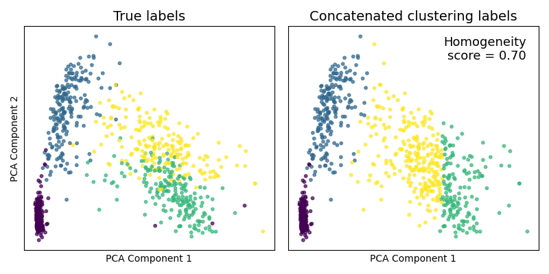
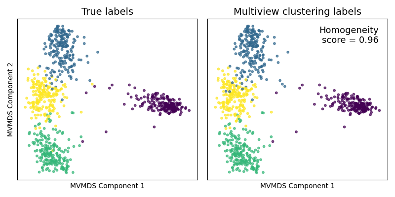
Now, assuming we are trying to group the samples into 4 clusters (as was much more obvious after using mvlearn's MVMDS dimensionality reduction method), we compare multiview spectral clustering (mvlearn.cluster.MultiviewSpectralClustering) to its singleview spectral clustering on the concatenated data. For multiview clustering, we use all 6 full views of data (not the dimensionality-reduced data). For singleview clustering, we concatenate these 6 full views into a single large matrix, the same as what we did before for PCA.

The true and predicted cluster labels are plotted on the prior reduced dimensionality embeddings. Since we have the true class labels, we assess the clustering accuracy with a homogeneity score. The multiview clustering clearly dominates its singleview approach.

def rearrange_labels(y_true, y_pred):
    """
    Rearranges labels among groups for better visual comparison
    """
    conf_mat = confusion_matrix(y_true, y_pred)
    maxes = np.argmax(conf_mat, axis=0)
    y_pred_new = np.zeros_like(y_pred)
    for i, new in enumerate(maxes):
        y_pred_new[y_pred == i] = new
    return y_pred_new


def plot_clusters(Xs, y_true, y_predicted, title, method):
    y_predicted = rearrange_labels(y, y_predicted)
    score = homogeneity_score(y, y_predicted)

    sca_kwargs = {'alpha': 0.7, 's': 10}
    f, axes = plt.subplots(1, 2, figsize=(8, 4))
    axes[0].scatter(Xs[:, 0], Xs[:, 1], c=y_true, **sca_kwargs)
    axes[0].set_title('True labels', fontsize=14)
    axes[1].scatter(Xs[:, 0], Xs[:, 1], c=y_predicted, **sca_kwargs)
    axes[1].set_title(title, fontsize=14)
    axes[1].annotate(
        f'Homogeneity\nscore = {score:.2f}', xy=(0.95, 0.85),
        xycoords='axes fraction', fontsize=13, ha='right')
    axes[0].set_ylabel(f'{method} Component 2')
    plt.setp(axes, xticks=[], yticks=[], xlabel=f'{method} Component 1')
    plt.tight_layout()
    plt.show()


# Cluster concatenated data
sv_clust = SpectralClustering(n_clusters=4, affinity='nearest_neighbors')
sv_labels = sv_clust.fit_predict(np.hstack(Xs))

plot_clusters(Xs_pca, y, sv_labels, 'Concatenated clustering labels', 'PCA')

# Cluster multiview data
mv_clust = MultiviewSpectralClustering(
    n_clusters=4, affinity='nearest_neighbors')
mv_labels = mv_clust.fit_predict(Xs)

plot_clusters(Xs_mvmds, y, mv_labels, 'Multiview clustering labels', 'MVMDS')

• 
•