An mvlearn case study: the Nutrimouse dataset

In this tutorial, we show how one may utilize various tools of mvlearn. We demonstrate applications to the mvlearn.datasets.load_nutrimouse dataset from a nutrition study on mice. The data measures 40 mice and has two views: expression levels of potentially relevant genes and concentrations of certain fatty acids. Each mouse has two labels: it's genetic type and diet.

1

P. Martin, H. Guillou, F. Lasserre, S. Déjean, A. Lan, J-M. Pascussi, M. San Cristobal, P. Legrand, P. Besse, T. Pineau. "Novel aspects of PPARalpha-mediated regulation of lipid and xenobiotic metabolism revealed through a nutrigenomic study." Hepatology, 2007.

# Authors: Ronan Perry
#
# License: MIT

Load the Nutrimouse dataset

import numpy as np
import matplotlib.pyplot as plt
import seaborn as sns
from mvlearn.datasets import load_nutrimouse

dataset = load_nutrimouse()
Xs = [dataset['gene'], dataset['lipid']]
y = np.vstack((dataset['genotype'], dataset['diet'])).T

print(f"Shapes of each view: {[X.shape for X in Xs]}")

Out:

Shapes of each view: [(40, 120), (40, 21)]

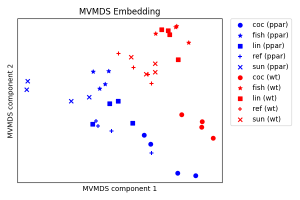
Embed using MVMDS

Multiview multidimensional scaling (mvlearn.embed.MVMDS) embeds multiview data into a single representation that captures information shared between both views. Embedding the two nutrimouse views, we can observe clear separation between the different genotypes and some of the diets too.

from mvlearn.embed import MVMDS  # noqa: E402

X_mvmds = MVMDS(n_components=2, num_iter=50).fit_transform(Xs)

diet_names = dataset['diet_names']
genotype_names = dataset['genotype_names']
plt.figure(figsize=(6, 4))
for genotype_idx, color in enumerate(('Blue', 'Red')):
    for diet_idx, marker in enumerate(('o', '*', 's', '+', 'x')):
        X_idx = np.where((y == (genotype_idx, diet_idx)).all(axis=1))
        label = diet_names[diet_idx] + f' ({genotype_names[genotype_idx]})'
        plt.scatter(*zip(*X_mvmds[X_idx]), c=color, label=label, marker=marker)

plt.xlabel('MVMDS component 1')
plt.ylabel('MVMDS component 2')
plt.title('MVMDS Embedding')
plt.xticks([])
plt.yticks([])
plt.legend(bbox_to_anchor=(1.04, 1), borderaxespad=0)
plt.tight_layout()
plt.show()

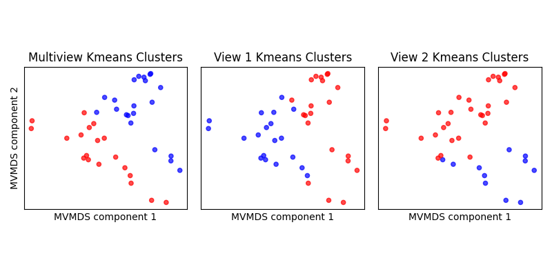
Cluster using Multiview KMeans

We can compare the estimated clusters from mvlearn.cluster.MultiviewKMeans to regular KMeans on each of the views. Multiview Kmeans clearly finds two clusters matching the two different genotype labels observed in the prior plots.

from mvlearn.cluster import MultiviewKMeans  # noqa: E402
from sklearn.cluster import KMeans  # noqa: E402

Xs_labels = MultiviewKMeans(n_clusters=2, random_state=0).fit_predict(Xs)
X1_labels = KMeans(n_clusters=2, random_state=0).fit_predict(Xs[0])
X2_labels = KMeans(n_clusters=2, random_state=0).fit_predict(Xs[1])

sca_kwargs = {'alpha': 0.7, 's': 20}
colors = np.asarray(['Red', 'Blue'])
f, axes = plt.subplots(1, 3, figsize=(8, 4))
axes[0].scatter(*zip(*X_mvmds), c=colors[Xs_labels], **sca_kwargs)
axes[0].set_title('Multiview Kmeans Clusters')
axes[1].scatter(*zip(*X_mvmds), c=colors[X1_labels], **sca_kwargs)
axes[1].set_title('View 1 Kmeans Clusters')
axes[2].scatter(*zip(*X_mvmds), c=colors[X2_labels], **sca_kwargs)
axes[2].set_title('View 2 Kmeans Clusters')

for ax in axes:
    ax.set_xlabel('MVMDS component 1')
    ax.set_xticks([])
    ax.set_yticks([])
    ax.set_aspect('equal')
axes[0].set_ylabel('MVMDS component 2')
axes[0].set_title('Multiview Kmeans Clusters')
plt.tight_layout()
plt.show()

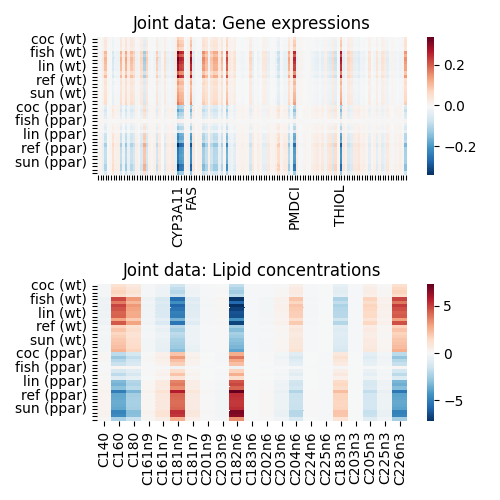
Decomposition using AJIVE

We can also apply joint decomposition tools to find features across views that are jointly related. Using mvlearn.decomposition.AJIVE, we can find genes and lipids that are jointly related.

from mvlearn.decomposition import AJIVE  # noqa: E402

ajive = AJIVE()
Xs_joint = ajive.fit_transform(Xs)

f, axes = plt.subplots(2, 1, figsize=(5, 5))
sort_idx = np.hstack((np.argsort(y[:20, 1]), np.argsort(y[20:, 1]) + 20))
y_ticks = [diet_names[j] + f' ({genotype_names[i]})' if idx %
           4 == 0 else '' for idx, (i, j) in enumerate(y[sort_idx])]

gene_ticks = [n if i in [31, 36, 76, 94] else '' for i,
              n in enumerate(dataset['gene_feature_names'])]
g = sns.heatmap(Xs_joint[0][sort_idx],
                yticklabels=y_ticks, cmap="RdBu_r", ax=axes[0],
                xticklabels=gene_ticks)
axes[0].set_title('Joint data: Gene expressions')

sns.heatmap(Xs_joint[1][sort_idx],
            yticklabels=y_ticks, cmap="RdBu_r", ax=axes[1],
            xticklabels=dataset['lipid_feature_names'])
axes[1].set_title('Joint data: Lipid concentrations')
plt.tight_layout()
plt.show()

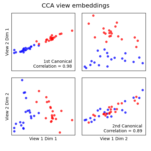
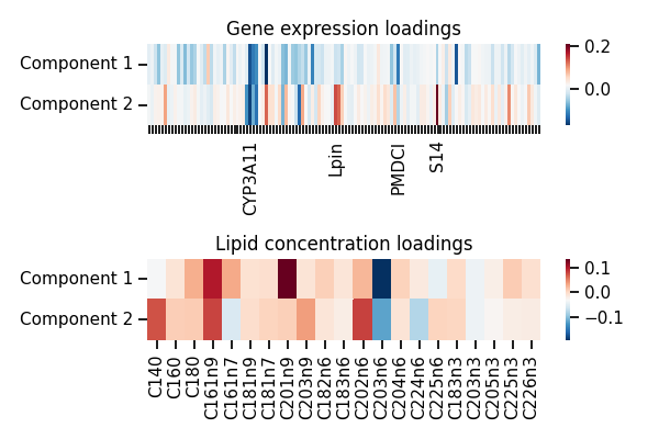
Inference using regularized CCA

Canonical Correlation Analysis (mvlearn.embed.CCA) finds separate linear projections of views which are maximally correlated. We can so embed the data jointly and observe that the first two embeddings are highly correlated and capture the differences between genetic types. One can use this to construct a single view for subsequent inference, or to examine the loading weights across views. Because the genetic expression data has more features than samples, we need to use regularization so as to not to trivially overfit.

from mvlearn.plotting import crossviews_plot  # noqa: E402
from mvlearn.embed import CCA  # noqa: E402

cca = CCA(n_components=2, regs=[0.9, 0.1])
Xs_cca = cca.fit_transform(Xs)

y_labels = [diet_names[j] + f' ({genotype_names[i]})' for (i, j) in y]
f, axes = crossviews_plot(
    Xs_cca, labels=np.asarray(['Red', 'Blue'])[y[:, 0]],
    ax_ticks=False, figsize=(5, 5), equal_axes=True,
    title='CCA view embeddings', scatter_kwargs=sca_kwargs,
    show=False)
corr1, corr2 = cca.canon_corrs(Xs_cca)
axes[0, 0].annotate(
    f'1st Canonical\nCorrelation = {corr1:.2f}', xy=(0.95, 0.05),
    xycoords='axes fraction', fontsize=10, ha='right')
axes[1, 1].annotate(
    f'2nd Canonical\nCorrelation = {corr2:.2f}', xy=(0.95, 0.05),
    xycoords='axes fraction', fontsize=10, ha='right')
plt.show()

f, axes = plt.subplots(2, 1, figsize=(6, 4))
gene_ticks = [n if i in [31, 57, 76, 88] else '' for i,
              n in enumerate(dataset['gene_feature_names'])]
g = sns.heatmap(cca.loadings_[0].T,
                yticklabels=['Component 1', 'Component 2'],
                cmap="RdBu_r", ax=axes[0],
                xticklabels=gene_ticks)
g.set_xticklabels(gene_ticks, rotation=90)
g.set_yticklabels(g.get_yticklabels(), va="center")
axes[0].set_title('Gene expression loadings')

g = sns.heatmap(cca.loadings_[1].T,
                yticklabels=['Component 1', 'Component 2'],
                cmap="RdBu_r", ax=axes[1],
                xticklabels=dataset['lipid_feature_names'])
g.set_yticklabels(g.get_yticklabels(), va="center")
axes[1].set_title('Lipid concentration loadings')
plt.tight_layout()
plt.show()

• 
•