Kernel MCCA (KMCCA) Tutorial

KMCCA is a variant of Canonical Correlation Analysis that can use a nonlinear kernel to uncover nonlinear correlations between views of data and thereby transform data into a lower dimensional space which captures the correlated information between views.

This tutorial runs KMCCA on two views of data. The kernel implementations, parameter 'ktype', are linear, polynomial and gaussian. Polynomial kernel has two parameters: 'constant', 'degree'. Gaussian kernel has one parameter: 'sigma'.

Useful information, like canonical correlations between transformed data and statistical tests for significance of these correlations can be computed using the get_stats() function of the KMCCA object.

When initializing KMCCA, you can also set the following parameters: the number of canonical components 'n_components', the regularization parameter 'reg', the decomposition type 'decomposition', and the decomposition method 'method'. There are two decomposition types: 'full' and 'icd'. In some cases, ICD will run faster than the full decomposition at the cost of performance. The only method as of now is 'kettenring-like'.

# Authors: Theodore Lee, Ronan Perry
# License: MIT

import numpy as np
from mvlearn.embed import KMCCA
from mvlearn.model_selection import train_test_split
from mvlearn.plotting import crossviews_plot
import warnings
warnings.filterwarnings("ignore")

# Function creates Xs, a list of two views of data with a linear relationship,
# polynomial relationship (2nd degree) and a gaussian (sinusoidal)
# relationship.


def make_data(kernel, N):
    # Define two latent variables (number of samples x 1)
    latvar1 = np.random.randn(N,)
    latvar2 = np.random.randn(N,)

    # Define independent components for each dataset
    # (number of observations x dataset dimensions)
    indep1 = np.random.randn(N, 4)
    indep2 = np.random.randn(N, 5)

    if kernel == "linear":
        x = 0.25 * indep1 + 0.75 * \
            np.vstack((latvar1, latvar2, latvar1, latvar2)).T
        y = 0.25 * indep2 + 0.75 * \
            np.vstack((latvar1, latvar2, latvar1, latvar2, latvar1)).T
        return [x, y]

    elif kernel == "poly":
        x = 0.25 * indep1 + 0.75 * \
            np.vstack((latvar1**2, latvar2**2, latvar1**2, latvar2**2)).T
        y = 0.25 * indep2 + 0.75 * \
            np.vstack((latvar1, latvar2, latvar1, latvar2, latvar1)).T
        return [x, y]

    elif kernel == "gaussian":
        t = np.random.uniform(-np.pi, np.pi, N)
        e1 = np.random.normal(0, 0.05, (N, 2))
        e2 = np.random.normal(0, 0.05, (N, 2))

        x = np.zeros((N, 2))
        x[:, 0] = t
        x[:, 1] = np.sin(3*t)
        x += e1

        y = np.zeros((N, 2))
        y[:, 0] = np.exp(t/4)*np.cos(2*t)
        y[:, 1] = np.exp(t/4)*np.sin(2*t)
        y += e2

        return [x, y]

Linear Kernel

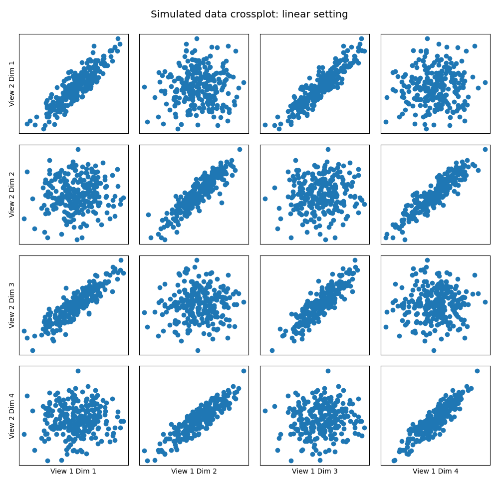
Here we show how KMCCA with a linear kernel can uncover the highly correlated latent distribution of the 2 views which are related with a linear relationship, and then transform the data into that latent space.

np.random.seed(1)
Xs = make_data('linear', 250)
Xs_train, Xs_test = train_test_split(Xs, test_size=0.3, random_state=42)

kmcca = KMCCA(n_components=4, regs=0.01)
scores = kmcca.fit_transform(Xs_test)

crossviews_plot(Xs, ax_ticks=False, ax_labels=True, equal_axes=True,
                title='Simulated data crossplot: linear setting')

crossviews_plot(scores, ax_ticks=False, ax_labels=True, equal_axes=True,
                title='Scores crossplot: linear KMCCA')

# Now, we assess the canonical correlations achieved on the testing data

print(f'Test data canonical correlations: {kmcca.canon_corrs(scores)}')

• 
• 

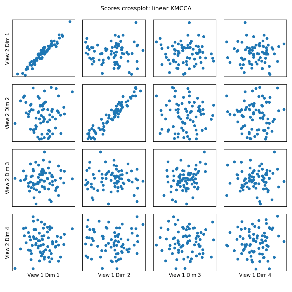
Out:

Test data canonical correlations: [0.96539304 0.95785531 0.24668706 0.07577206]

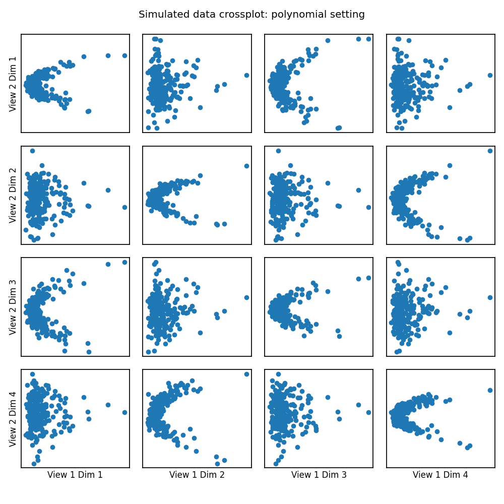
Polynomial Kernel

# Here we show how KMCCA with a polynomial kernel can uncover the highly
# correlated latent distribution of the 2 views which are related with a
# polynomial relationship, and then transform the data into that latent space.


Xs = make_data("poly", 250)
Xs_train, Xs_test = train_test_split(Xs, test_size=0.3, random_state=42)

kmcca = KMCCA(
    kernel="poly", kernel_params={'degree': 2.0, 'coef0': 0.1},
    n_components=4, regs=0.01)
scores = kmcca.fit(Xs_train).transform(Xs_test)

crossviews_plot(Xs, ax_ticks=False, ax_labels=True, equal_axes=True,
                title='Simulated data crossplot: polynomial setting')

crossviews_plot(scores, ax_ticks=False, ax_labels=True, equal_axes=True,
                title='Scores crossplot: polynomial KMCCA')

# Now, we assess the canonical correlations achieved on the testing data

print(f'Test data canonical correlations: {kmcca.canon_corrs(scores)}')

• 
• 

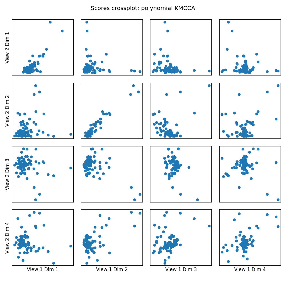
Out:

Test data canonical correlations: [ 0.82270834  0.9629903  -0.34427048  0.50149524]

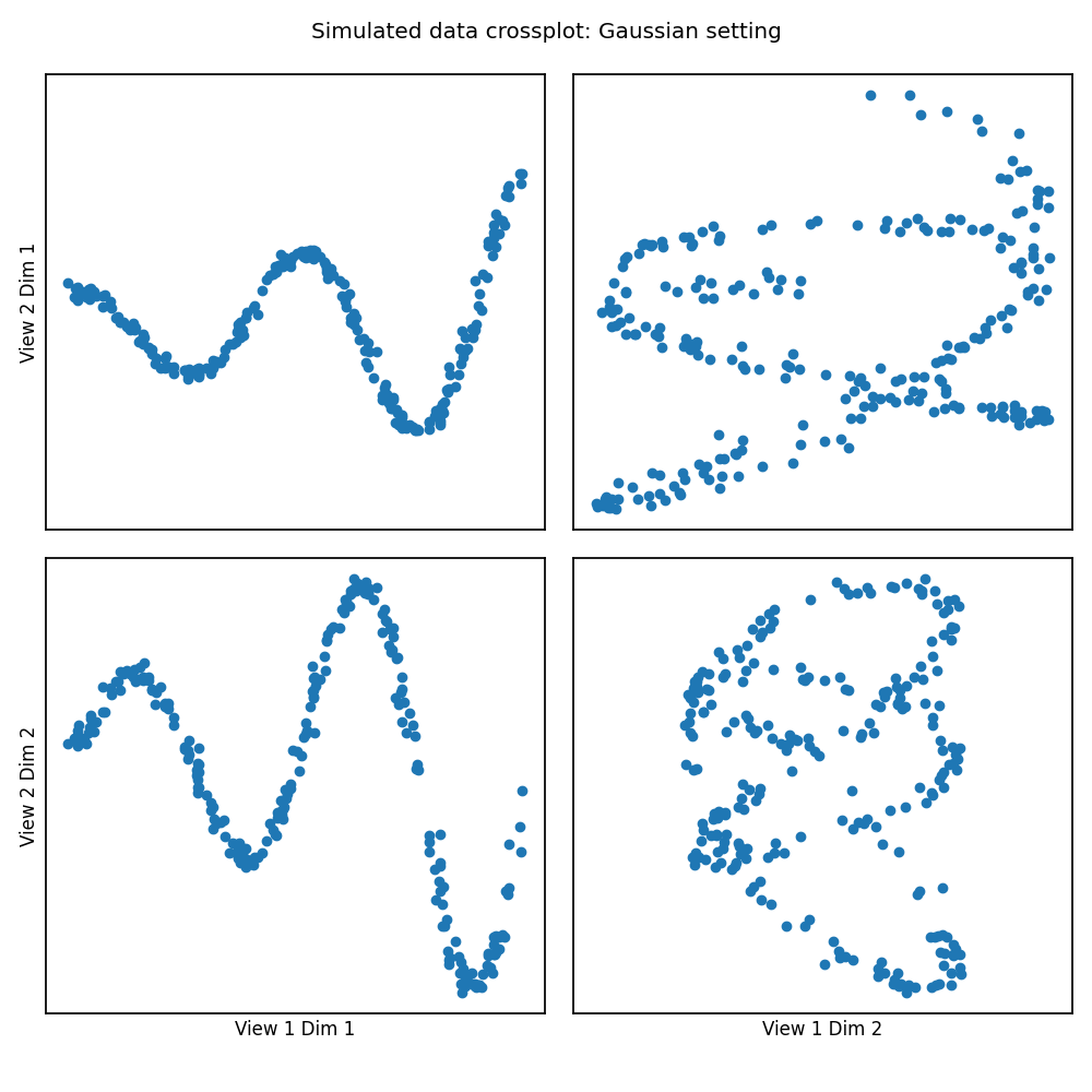
Gaussian Kernel

# Here we show how KMCCA with a gaussian kernel can uncover the highly
# correlated latent distribution of the 2 views which are related with a
# sinusoidal relationship, and then transform the data into that latent space.


Xs = make_data("gaussian", 250)
Xs_train, Xs_test = train_test_split(Xs, test_size=0.3, random_state=42)

kmcca = KMCCA(
    kernel="rbf", kernel_params={'gamma': 1}, n_components=2, regs=0.01)
scores = kmcca.fit(Xs_train).transform(Xs_test)

crossviews_plot(Xs, ax_ticks=False, ax_labels=True, equal_axes=True,
                title='Simulated data crossplot: Gaussian setting')

crossviews_plot(scores, ax_ticks=False, ax_labels=True, equal_axes=True,
                title='Scores crossplot: Gaussian KMCCA')

# Now, we assess the canonical correlations achieved on the testing data

print(f'Test data canonical correlations: {kmcca.canon_corrs(scores)}')

• 
• 

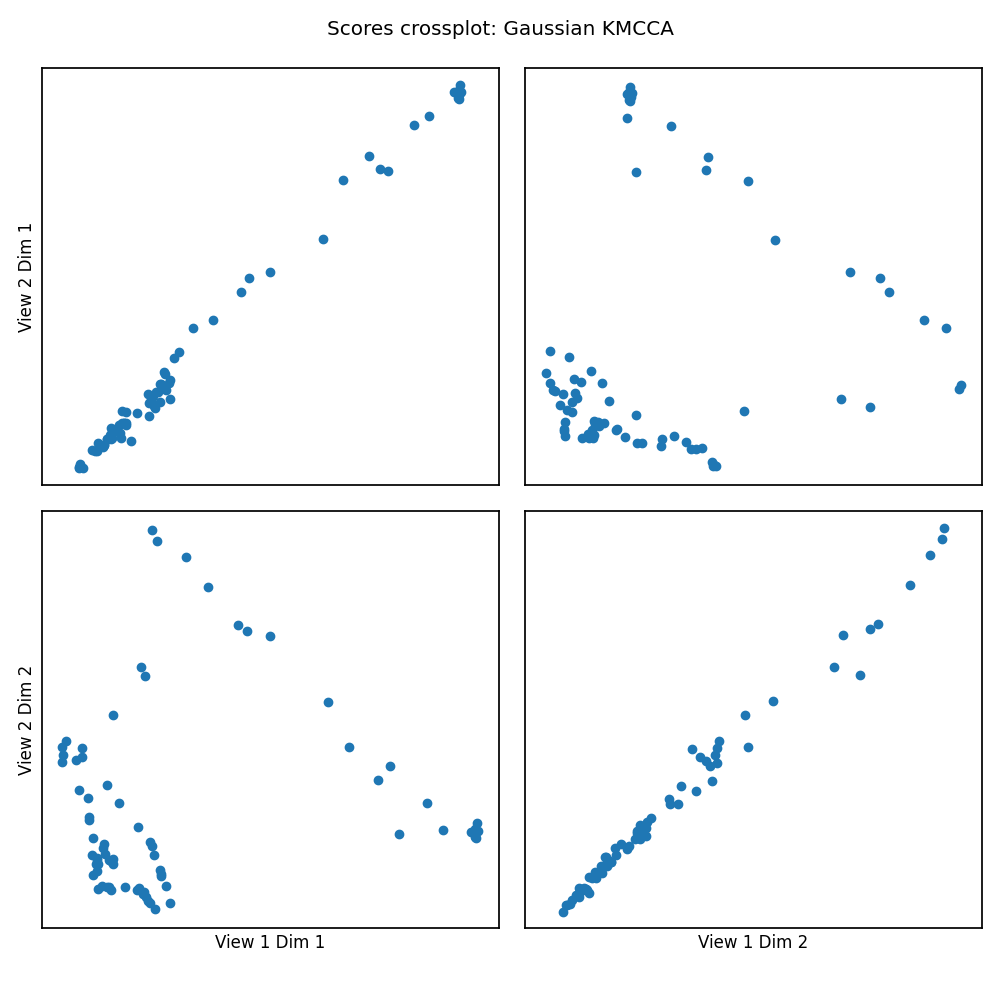
Out:

Test data canonical correlations: [0.9966364  0.99352519]