Multiview Spectral Clustering Tutorial

This tutorial demonstrates how to use multiview spectral clustering to cluster multiview datasets, showing results on both synthetic data and the UCI multiview digits dataset.

# License: MIT

import warnings
import numpy as np
import matplotlib.pyplot as plt

from sklearn.cluster import SpectralClustering
from sklearn.metrics import normalized_mutual_info_score as nmi_score
from sklearn.datasets import make_moons

from mvlearn.datasets import load_UCImultifeature
from mvlearn.cluster import MultiviewSpectralClustering
from mvlearn.plotting import quick_visualize

warnings.simplefilter('ignore')  # Ignore warnings
RANDOM_SEED = 10

Plotting and moon data generating functions

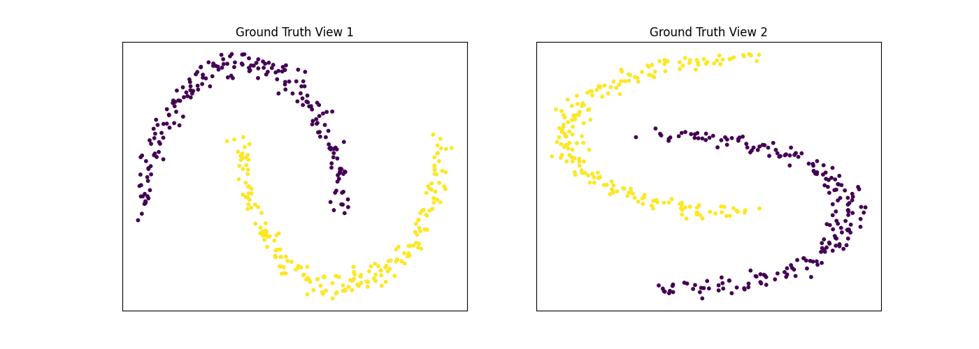
For this example, we use the sklearn make_moons function to make two interleaving half circles in two views. We then use spectral clustering to separate the two views. As we can see below, multi-view spectral clustering is capable of effectively clustering non-convex cluster shapes, similarly to its single-view analog.

The following function plots both views of data given a dataset and corresponding labels.

def display_plots(pre_title, data, labels):
    # plot the views
    fig, ax = plt.subplots(1, 2, figsize=(14, 5))
    dot_size = 10
    ax[0].scatter(data[0][:, 0], data[0][:, 1], c=labels, s=dot_size)
    ax[0].set_title(pre_title + ' View 1')
    ax[0].axes.get_xaxis().set_visible(False)
    ax[0].axes.get_yaxis().set_visible(False)

    ax[1].scatter(data[1][:, 0], data[1][:, 1], c=labels, s=dot_size)
    ax[1].set_title(pre_title + ' View 2')
    ax[1].axes.get_xaxis().set_visible(False)
    ax[1].axes.get_yaxis().set_visible(False)

    plt.show()


# A function to generate the moons data
def create_moons(seed, num_per_class=200):
    np.random.seed(seed)
    data = []
    labels = []

    for view in range(2):
        v_dat, v_labs = make_moons(num_per_class*2,
                                   random_state=seed + view, noise=0.05,
                                   shuffle=False)
        if view == 1:
            v_dat = v_dat[:, ::-1]

        data.append(v_dat)
    for ind in range(len(data)):
        labels.append(ind * np.ones(num_per_class,))
    labels = np.concatenate(labels)

    return data, labels


# Generating the data
m_data, labels = create_moons(RANDOM_SEED)
n_class = 2

Single-view spectral clustering

Cluster each view separately

s_spectral = SpectralClustering(n_clusters=n_class,
                                affinity='nearest_neighbors',
                                random_state=RANDOM_SEED, n_init=10)
s_clusters_v1 = s_spectral.fit_predict(m_data[0])
s_clusters_v2 = s_spectral.fit_predict(m_data[1])

# Concatenate the multiple views into a single view
s_data = np.hstack(m_data)
s_clusters = s_spectral.fit_predict(s_data)

# Compute nmi between true class labels and single-view cluster labels
s_nmi_v1 = nmi_score(labels, s_clusters_v1)
s_nmi_v2 = nmi_score(labels, s_clusters_v2)
s_nmi = nmi_score(labels, s_clusters)
print('Single-view View 1 NMI Score: {0:.3f}\n'.format(s_nmi_v1))
print('Single-view View 2 NMI Score: {0:.3f}\n'.format(s_nmi_v2))
print('Single-view Concatenated NMI Score: {0:.3f}\n'.format(s_nmi))

Out:

Single-view View 1 NMI Score: 1.000

Single-view View 2 NMI Score: 0.496

Single-view Concatenated NMI Score: 1.000

Multiview spectral clustering

Use the MultiviewSpectralClustering instance to cluster the data

m_spectral = MultiviewSpectralClustering(n_clusters=n_class,
                                         affinity='nearest_neighbors',
                                         max_iter=12, random_state=RANDOM_SEED,
                                         n_init=10)
m_clusters = m_spectral.fit_predict(m_data)

# Compute nmi between true class labels and multi-view cluster labels
m_nmi = nmi_score(labels, m_clusters)
print('Multi-view NMI Score: {0:.3f}\n'.format(m_nmi))

Out:

Multi-view NMI Score: 1.000

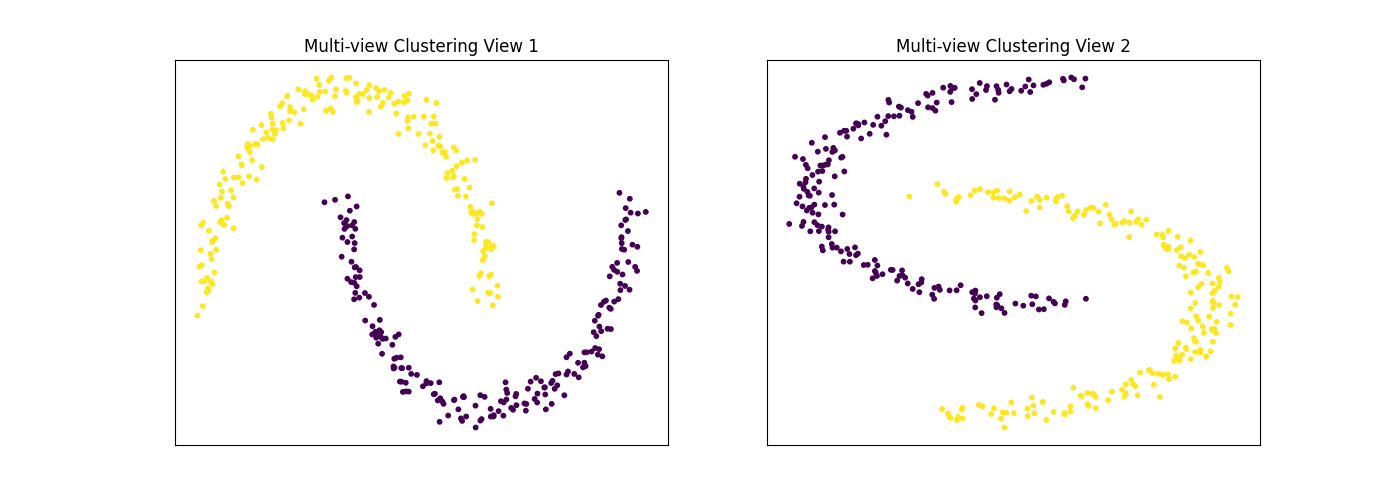
Plots of clusters produced by multi-view spectral clustering and the true clusters

We will display the clustering results of the Multi-view spectral clustering algorithm below, along with the true class labels.

display_plots('Ground Truth', m_data, labels)
display_plots('Multi-view Clustering', m_data, m_clusters)

• 
• 

Performance on the UCI Digits Multiple Features data set with 2 views

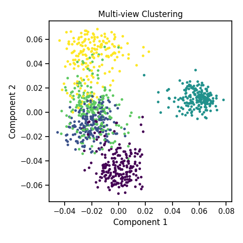
Here we will compare the performance of the Multi-view and Single-view versions of spectral clustering. We will evaluate the purity of the resulting clusters from each algorithm with respect to the class labels using the normalized mutual information metric.

As we can see, Multi-view clustering produces clusters with higher purity compared to those produced by Single-view clustering for all 3 input types.

# Load dataset along with labels for digits 0 through 4
n_class = 5
Xs, labels = load_UCImultifeature(
    select_labeled=list(range(n_class)), views=[0, 1])

Singleview spectral clustering

Cluster each view separately

s_spectral = SpectralClustering(n_clusters=n_class, random_state=RANDOM_SEED,
                                n_init=100)

for i in range(len(Xs)):
    s_clusters = s_spectral.fit_predict(Xs[i])
    s_nmi = nmi_score(labels, s_clusters, average_method='arithmetic')
    print('Single-view View {0:d} NMI Score: {1:.3f}\n'.format(i + 1, s_nmi))

# Concatenate the multiple views into a single view and produce clusters
X = np.hstack(Xs)
s_clusters = s_spectral.fit_predict(X)

s_nmi = nmi_score(labels, s_clusters)
print('Single-view Concatenated NMI Score: {0:.3f}\n'.format(s_nmi))

Out:

Single-view View 1 NMI Score: 0.620

Single-view View 2 NMI Score: 0.007

Single-view Concatenated NMI Score: 0.007

Multiview spectral clustering

Use the MultiviewSpectralClustering instance to cluster the data

m_spectral1 = MultiviewSpectralClustering(n_clusters=n_class,
                                          random_state=RANDOM_SEED,
                                          n_init=10)
m_clusters1 = m_spectral1.fit_predict(Xs)

# Compute nmi between true class labels and multi-view cluster labels
m_nmi1 = nmi_score(labels, m_clusters1)
print('Multi-view NMI Score: {0:.3f}\n'.format(m_nmi1))

Out:

Multi-view NMI Score: 0.872

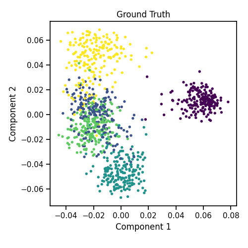
Plots of clusters produced by multi-view spectral clustering and the true clusters

We will display the clustering results of the Multi-view spectral clustering algorithm below, along with the true class labels.

quick_visualize(Xs, labels=labels, title='Ground Truth',
                scatter_kwargs={'s': 8})
quick_visualize(Xs, labels=m_clusters1, title='Multi-view Clustering',
                scatter_kwargs={'s': 8})

• 
•