Generalized Canonical Correlation Analysis (GCCA) Tutorial

In this tutorial we demonstrate the use of GCCA to uncover latent correlated information across views when we have more than 2 views. In this case, we use 3 views from the UCI Multiple Features Dataset.

# License: MIT

from mvlearn.datasets import load_UCImultifeature
from mvlearn.embed import GCCA
from mvlearn.plotting import crossviews_plot

Load Data

We load three views from the UCI handwritten digits multi-view data set. Specificallym the Profile correlations, Karhunen-Love coefficients, and pixel averages from 2x3 windows.

# Load the data
Xs, y = load_UCImultifeature(views=[1, 2, 3])

# Inspect the dataset
print(f'There are {len(Xs)} views.')
print(f'There are {Xs[0].shape[0]} observations')
print(f'The feature sizes are: {[X.shape[1] for X in Xs]}')

Out:

There are 3 views.
There are 2000 observations
The feature sizes are: [216, 64, 240]

Embed Views

# Create GCCA object and embed the
gcca = GCCA()
Xs_latents = gcca.fit_transform(Xs)

print(f'The feature sizes are: {[X.shape[1] for X in Xs_latents]}')

Out:

The feature sizes are: [5, 5, 5]

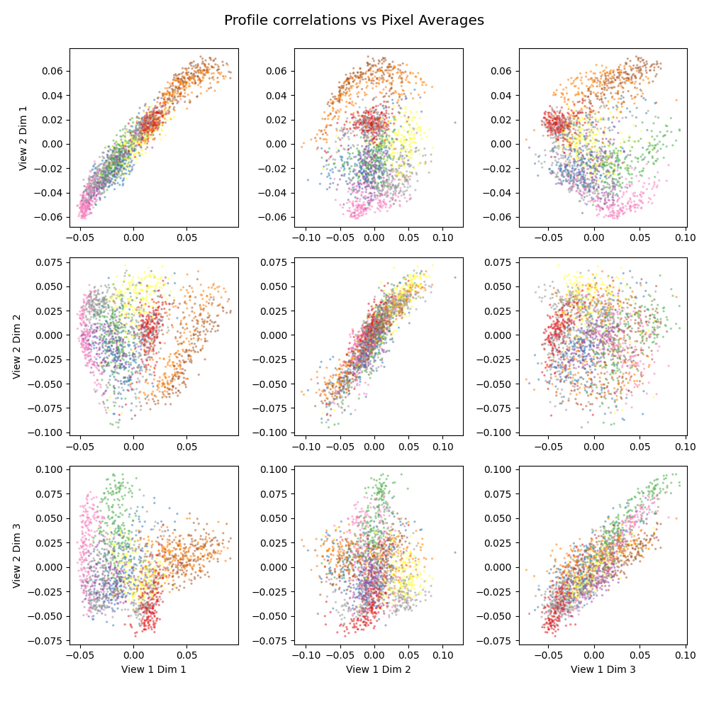
Plot the first two views against each other

The top three dimensions from the latents spaces of the profile correlation and pixel average views are plotted against each other. However, their latent spaces are influenced the the Karhunen-Love coefficients, not plotted.

crossviews_plot(Xs_latents[[0, 2]], dimensions=[0, 1, 2], labels=y,
                cmap='Set1', title='Profile correlations vs Pixel Averages',
                scatter_kwargs={'alpha': 0.4, 's': 2.0})