Comparing CCA Variants

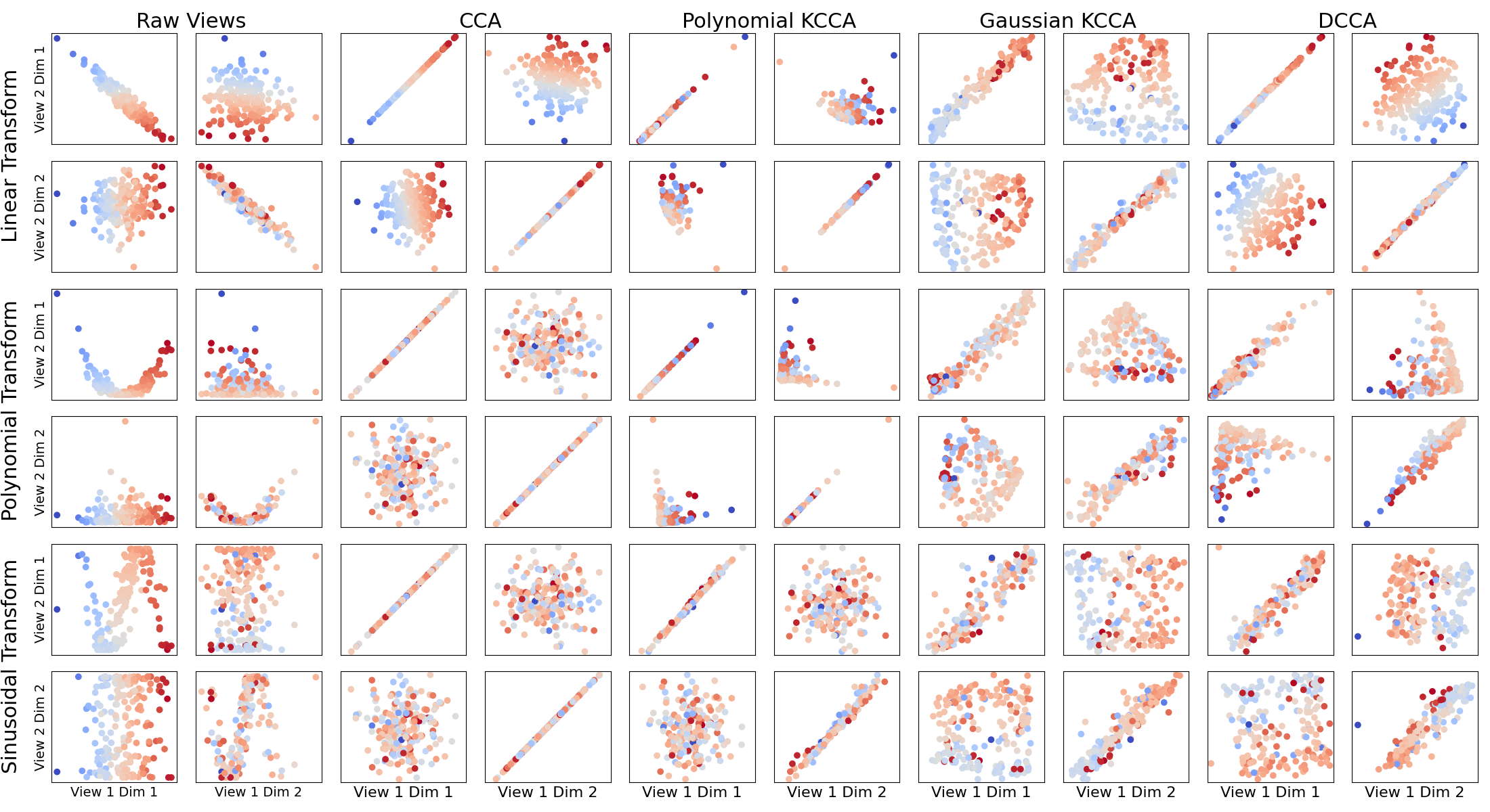
This tutorial shows a comparison of Canonical Correlation Analysis (CCA), Kernel CCA (KCCA) with two different types of kernel, and Deep CCA (DCCA). CCA is equivalent to KCCA with a linear kernel. Each learns kernels suitable for different situations. The point of this tutorial is to illustrate, in toy examples, the rough intuition as to when such methods work well and find highly correlated projections.

The simulated latent data has two signal dimensions draw from independent Gaussians. Two views of data were derived from this.

• View 1: The latent data.

• View 2: A transformation of the latent data.

To each view, two additional independent Gaussian noise dimensions were added.

Each 2x2 grid of subplots in the figure corresponds to a transformation and either the raw data or a CCA variant. The x-axes are the data from view 1 and the y-axes are the data from view 2. Plotted are the correlations between the signal dimensions of the raw views and the top two components of each view after a CCA variant transformation. Linearly correlated plots on the diagonals of the 2x2 grids indicate that the CCA method was able to successfully learn the underlying functional relationship between the two views.

# Author: Ronan Perry
# License: MIT

from mvlearn.embed import CCA, KMCCA, DCCA
from mvlearn.datasets import make_gaussian_mixture
import numpy as np
import matplotlib.pyplot as plt
import matplotlib
import seaborn as sns
import warnings
warnings.filterwarnings("ignore")

# GMM settings
n_samples = 200
centers = [[0, 0], [0, 0]]
covariances = 4*np.array([np.eye(2), np.eye(2)])
transforms = ['linear', 'poly', 'sin']

Xs_train_sets = []
Xs_test_sets = []
for transform in transforms:
    Xs_train, _ = make_gaussian_mixture(
        n_samples, centers, covariances, transform=transform, noise=0.25,
        noise_dims=2, random_state=41)
    Xs_test, _, latents = make_gaussian_mixture(
        n_samples, centers, covariances, transform=transform, noise=0.25,
        noise_dims=2, random_state=42, return_latents=True)

    Xs_train_sets.append(Xs_train)
    Xs_test_sets.append(Xs_test)


# Plotting parameters
labels = latents[:, 0]
cmap = matplotlib.colors.ListedColormap(
    sns.diverging_palette(240, 10, n=len(labels), center='light').as_hex())
cmap = 'coolwarm'

method_labels = \
    ['Raw Views', 'CCA', 'Polynomial KCCA', 'Gaussian KCCA', 'DCCA']
transform_labels = \
    ['Linear Transform', 'Polynomial Transform', 'Sinusoidal Transform']

input_size1 = Xs_train_sets[0][0].shape[1]
input_size2 = Xs_train_sets[0][1].shape[1]
outdim_size = min(Xs_train_sets[0][0].shape[1], 2)
layer_sizes1 = [256, 256, outdim_size]
layer_sizes2 = [256, 256, outdim_size]
methods = [
    CCA(regs=0.1, n_components=2),
    KMCCA(kernel='poly', regs=0.1, kernel_params={'degree': 2, 'coef0': 0.1},
          n_components=2),
    KMCCA(kernel='rbf', regs=0.1, kernel_params={'gamma': 1/4},
          n_components=2),
    DCCA(input_size1, input_size2, outdim_size, layer_sizes1, layer_sizes2,
         epoch_num=400)
]

fig, axes = plt.subplots(3 * 2, 5 * 2, figsize=(22, 12))
sns.set_context('notebook')

for r, transform in enumerate(transforms):
    axs = axes[2 * r:2 * r + 2, :2]
    for i, ax in enumerate(axs.flatten()):
        dim2 = int(i / 2)
        dim1 = i % 2
        ax.scatter(
            Xs_test_sets[r][0][:, dim1],
            Xs_test_sets[r][1][:, dim2],
            cmap=cmap,
            c=labels,
        )
        ax.set_xticks([], [])
        ax.set_yticks([], [])
        if dim1 == 0:
            ax.set_ylabel(f"View 2 Dim {dim2+1}", fontsize=14)
        if dim1 == 0 and dim2 == 0:
            ax.text(-0.4, -0.1, transform_labels[r], transform=ax.transAxes,
                    fontsize=22, rotation=90, verticalalignment='center')
        if dim2 == 1 and r == len(transforms)-1:
            ax.set_xlabel(f"View 1 Dim {dim1+1}", fontsize=14)
        if i == 0 and r == 0:
            ax.set_title(method_labels[r],
                         {'position': (1.11, 1), 'fontsize': 22})

    for c, method in enumerate(methods):
        axs = axes[2*r: 2*r+2, 2*c+2:2*c+4]
        Xs = method.fit(Xs_train_sets[r]).transform(Xs_test_sets[r])
        for i, ax in enumerate(axs.flatten()):
            dim2 = int(i / 2)
            dim1 = i % 2
            ax.scatter(
                Xs[0][:, dim1],
                Xs[1][:, dim2],
                cmap=cmap,
                c=labels,
            )
            if dim2 == 1 and r == len(transforms)-1:
                ax.set_xlabel(f"View 1 Dim {dim1+1}", fontsize=16)
            if i == 0 and r == 0:
                ax.set_title(method_labels[c + 1], {'position': (1.11, 1),
                             'fontsize': 22})
            ax.axis("equal")
            ax.set_xticks([], [])
            ax.set_yticks([], [])

plt.tight_layout()
plt.subplots_adjust(wspace=0.15, hspace=0.15)
plt.show()